Rules for creating formulas in excel. Filtering data in the list. Applying color and patterns

3.Principles of working in Excel

3.1 Working with formulas

Formula is a special Excel tool designed for calculations and data analysis. A formula begins with an "=" sign, followed by operands and operators. The simplest example of creating a formula can be represented as follows: first, the “=” sign is entered into the cell, then a certain number, after that, an arithmetic sign (+, -, * or /), etc. The process of entering the formula is completed by pressing the Enter key - as a result, the result of the formula calculation will be displayed in the cell. If you select this cell, then the entered formula will be shown in the formula bar. However, this way of creating formulas is not always acceptable. This is due to the fact that often for calculations it is necessary to use not just specific numerical values, but the data in certain cells. In this case, the addresses of the corresponding cells are indicated in the formula. If necessary, any previously created formula can be edited. To do this, select the appropriate cell and enter the required changes in the formula bar, and then press the Enter key. You can also change the formula in the cell itself: to switch to edit mode, you need to place the cursor on it and press the F2 key. The program features include entering a formula simultaneously in several cells. To do this, select the required range, then enter the necessary formula in the first cell and press the Ctrl + Enter key combination. The formula can be copied to the clipboard and pasted anywhere on the worksheet. In this case, all used links (cell addresses) in the source formula will be automatically replaced in the destination formula with similar links corresponding to the new placement of the formula. For example, if you enter the formula =B2+C1 in cell A1, then copy it to the clipboard and paste it into cell A2, then the formula will look like this: =B2+C2. If necessary, do not copy, but move the formula from one cell to another, select this cell, move the mouse pointer to any of its borders so that it turns into a cross, press the left mouse button and, holding it, drag the formula to the desired location. If you need to copy to the clipboard and then paste in the required place not a formula, but only the value obtained as a result of its calculation, you should select the cell, then copy its contents to the clipboard, move the cursor to the place where you want to paste the data, and select in context menu item Special insert. As a result, a window of the same name will open, in which you should set the switch Insert into position values and press OK. In this window, you can select other modes for pasting the contents of the clipboard. Sometimes it may be necessary to quickly view all the formulas that are in the cells of a worksheet. To do this, run the command Service Options, in the opened window Options tab View check the box formulas and press the button OK. As a result, in cells containing formulas, the formulas themselves will be displayed, and not the result of their calculation. To return to the original display mode, uncheck this box. To delete a formula, just select the corresponding cell and press the Delete key. If the formula is erased by mistake, then immediately after deletion it can be restored in its original place by pressing the key combination Ctrl + Z.

3.2 Working with functions

A function is a formula that was originally created and embedded in the program, which allows you to perform calculations on given values ​​and in a certain order. Each function includes the following components: sign "=", name (SUM, AVERAGE, COUNT, MAX, etc.) and arguments. The arguments used depend on the particular function. Arguments can be numbers, links, formulas, text, booleans, etc. Each function has its own syntax, which must be followed. Even a slight deviation from the syntax will lead to erroneous calculations or even to the impossibility of calculation. Functions can be entered either manually or automatically. For automatic input, the function wizard is intended, called using the command Insert Function. You can type the function manually in the formula bar (you must first select the cell in which data is entered) in the following order: first, an equal sign is indicated, then the name of the function, and after that, a list of arguments that are enclosed in parentheses and separated by a semicolon. For example, you need to find the sum of the numbers in cells A1, B2, C5. To do this, enter the following expression in the formula bar: =SUM(A1;B2;C5). In this case, the name is entered in Russian letters, and the arguments, which are cell addresses, are in Latin. After pressing the Enter key, the result of the calculation will be displayed in the active cell. Any function can be used as an argument for some other function. This is called function nesting. The program features include up to seven levels of function nesting.

3.3 Working with charts

One of the most useful features Excel programs is a diagramming engine. In general, a chart is a visual graphical representation of the available data. The construction of the diagram is carried out on the basis of the information on the worksheet. At the same time, it can be located both on the same sheet with the data on the basis of which it is built (such a chart is called embedded), and on separate sheet(in this case, a chart sheet is created). The chart is inextricably linked to the source data and is automatically updated accordingly whenever it changes. To switch to the diagram construction mode, use the main menu command Insert Diagram. When executed, the Chart Wizard window opens:
Before using this command, it is recommended to select a range with data on the basis of which the chart will be built. But this range can be specified (or edited) later, at the second step of constructing the chart. The first step in building a chart is to choose its type. The program features include the construction of a variety of charts: histograms, graphs, pie charts, scatter charts, petal charts, bubble charts, etc. On the tab Standard a list of standard diagrams is given. If none of them satisfies the user's requirements, you can choose a custom chart by going to the tab non-standard. To select the desired chart, you need to select its type in the left part of any of the tabs, and the presentation option in the right part. If when executing the command Insert Diagram If a data range has been selected on the basis of which a chart should be built, then in the Chart Wizard window, using the button View result you can see how the diagram will look like with the this moment settings. The finished chart is displayed on the right side of the tab only when this button is pressed. To go to the second stage of plotting the diagram, press the button Further. The chart creation process can be ended at any time by clicking the Finish button. As a result, a diagram corresponding to the specified settings will be created. If before executing the command Insert Diagram range with data was not specified, then at the second step in the field Range it should be specified. Here, if necessary, you can edit the previously specified data range. With switch ranks the required option for constructing data series is selected: by rows or by columns of the selected range. On the tab Row you can add data series to and remove data series from the chart. To add a row, click the button Add and in the field on the right Values Specify the range of data to be used when plotting the chart. To remove a row from the list, select its name and press the button Delete. In this case, you must be careful, because the program does not prompt you to confirm the deletion operation. Push button Further the transition to the third stage of diagram construction is carried out. The window that appears consists of the following tabs: Titles(opens by default) axes, grid lines, Legend, Data Signatures And data table. The number of tabs in the window depends on the selected chart type. On the tab Titles in the corresponding fields, the name of the chart and its axes are entered from the keyboard. The entered values ​​are immediately displayed in the viewing area on the right. The fields on this tab are optional. On the tab axes the presence of axes (horizontal and vertical) on the diagram is configured. If the display of an axis is disabled, then the chart will not have the axis itself and the values ​​located on it. To enable the display of the axes, the checkboxes X-axis (categories) and Y-axis (values) must be checked. They are set by default. To set up the grid lines of the chart, use the tab grid lines. Here, for each axis, by setting the appropriate checkboxes, you can enable the display of main and intermediate lines. On the tab Legend you can control the display of the chart legend. A legend is a list of series in a chart, with the color of each series indicated. To enable the display of the legend, you need to check the box Add legend(it is installed by default). This makes the switch available. Accommodation, which specifies the location of the legend in relation to the chart: bottom, top right, top, right, and left. On the tab Data Signatures chart labels are configured. For example, when checking the checkbox values the diagram will show the source data on which it is based. If you check the box row names, then its name will be displayed above each data series (the names of the series are displayed in accordance with the list of series that was formed at the second step of constructing a chart on the tab Row). If on the tab data table check the box of the same name, then immediately below the diagram a table with the initial data on the basis of which the diagram is built will be displayed. When you press a button Further the transition to the fourth, final stage of the diagram construction is performed.


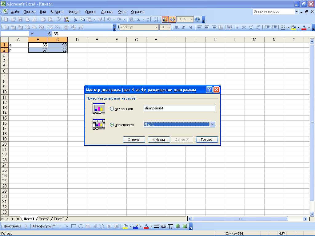
At this step, the location of the diagram is determined. If the switch is set to separate, then after pressing the button Ready a separate worksheet will be automatically generated for the chart. By default, this sheet will be named Diagram 1, but you can change it if necessary. The process of building a diagram is completed by pressing the button Ready. If the switch is set to available, then in the drop-down list located on the right, select a worksheet from those available in the current workbook on which the chart will be placed. In this way, you can build a wide variety of charts, depending on the needs of the user. To quickly navigate to the data on which the chart was built, you need to right-click on it and select the item in the context menu that opens. Initial data. As a result, the diagram wizard window will open in the second step, in the field Range which will indicate the boundaries of the range with the source data. In addition, after executing this command, a range with initial values ​​will be selected on the worksheet. If necessary, you can change the location of the chart at any time. To do this, right-click on it and select Placement from the context menu that opens. This will bring up a dialog box (step 4) in which you can specify a new chart placement order. To remove a chart from a worksheet, select it with the mouse button and press the Delete key. If you need to delete a chart located on a separate sheet, then right-click on the label of the chart sheet and select the command in the context menu that opens. Delete. In this case, the program will issue an additional request to confirm the deletion operation.

3.3.1. Changing the appearance of a 3-D chart

E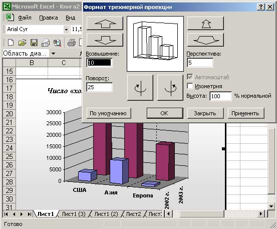

if you are not satisfied appearance of the resulting volumetric diagram, then a number of its parameters are easy to change. To do this, select a chart and use the command Diagram 3D view- the Format 3D Projection window will open, where you can make changes. When choosing new parameter values, you should pay attention to the button Apply, with which you can see changes in the diagram without closing the editing window. You can also change the elevation and rotation angle of the diagram using the mouse by clicking it in one of the corners of the diagram and dragging any of the selected corners as necessary. This process is more convenient to carry out with the Ctrl key pressed to make the internal contours of the diagram visible.

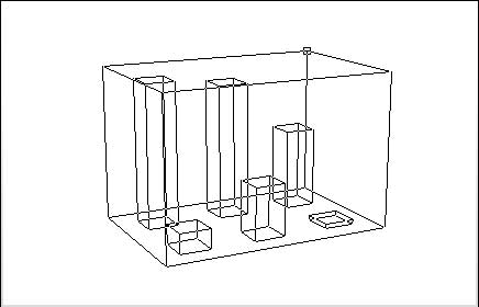
3.4 Inserting, editing and deleting notes

The program implements the ability to add to any cell the necessary text comment - notes. The meaning of this operation is that the note can be displayed either permanently or only when the mouse pointer is hovered over the corresponding cell. You can control the display of notes in the window Options tab View with switch Notes.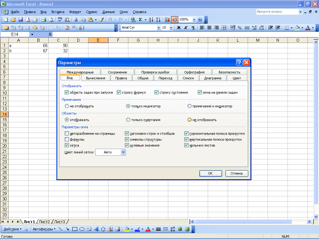

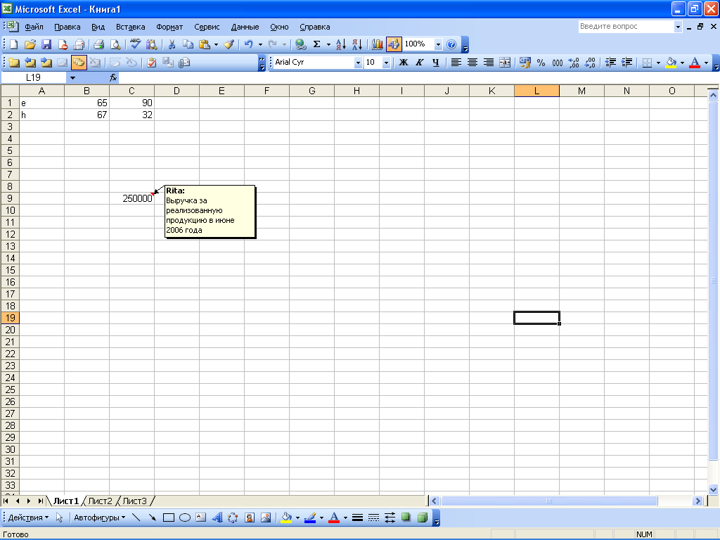
Note Example

To add a comment to a cell, you need to right-click on it and select the item in the context menu that opens. Add note. You can also place the cursor in a cell and use the main menu command Insert Note. As a result, a note window will open, in which the username will be displayed by default. Note text can be absolutely arbitrary, it is typed from the keyboard. To complete the entry of a note, just click anywhere on the worksheet. A previously created note can be edited at any time. To do this, right-click on the cell with the note and select Edit Note from the context menu. As a result, a note window will open in which you can make the required changes. When editing is complete, click anywhere on the sheet to make the note box disappear. To delete a note, right-click on the corresponding cell and in the context menu that opens, execute the command Delete note. In this case, you should be careful, because the program does not issue an additional request to confirm the deletion operation. If necessary, you can select all cells of the current worksheet that have comments - to do this, press the key combination Ctrl + Shift + O. To remove notes from all cells of the sheet, you need to select them using the combination Ctrl + Shift + O, then right-click on any of these cells and select the item from the context menu Delete note.

3.5 Using AutoShapes

Sometimes in the course of work, it becomes necessary to add graphic objects to the document, designed to highlight a certain fragment of the worksheet, create a diagram or callout, point to something with an arrow, etc. To facilitate this work, the program implements the possibility of using autoshapes. Its essence lies in the fact that the user selects the required figure from the proposed list and then marks the boundaries within which it should be placed with the mouse pointer. You can access the AutoShapes available in Excel using the toolbar Drawing. To enable its display, you need to run the command View Toolbars Drawing. By default, this panel is located at the bottom of the program window. To work with autoshapes on the toolbar Drawing designed button AutoShapes. When pressed, this menu opens: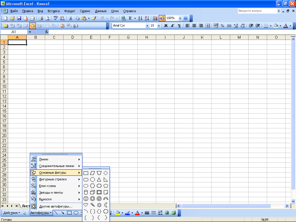


This menu provides access to the autoshapes available in the program. All autoshapes are combined into thematic submenu groups: Lines, Connectors, Basic Shapes, Curly Arrows, Flowchart, Stars and Ribbons, Callouts, Other AutoShapes. To insert an AutoShape into a document, you need to select it in the corresponding submenu, then move the mouse pointer to the place on the worksheet where the AutoShape should be inserted, and click the mouse button. If necessary, you can stretch the autoshape to any size required by the user. To do this, after selecting the autoshape, press the mouse button and, holding it, move the pointer in the required direction. If necessary, using the tools of the Drawing panel, you can additionally shape the autoshape (for example, paint the object and its outline with different colors, change the thickness and type of the line). Any number of AutoShapes of arbitrary size can be inserted into any document, depending on the needs of the user.

3.6 Setting up and using a data entry form

When working with large amounts of information, it may be necessary to fill in a wide variety of tables of considerable size. For quick filling large tables it is recommended to use a data entry form that the user configures independently depending on the current task. Suppose we need to fill in a table with three columns called Profit, Loss and Taxes. This table is located starting from cell A1. First you need to type the names of the columns of the table. In our case, in cell A1 we will enter the value of Profit, in cell B1 - Losses, in cell C1 - Taxes. Then you need to select these cells and run the command Data Form- as a result, this message will appear: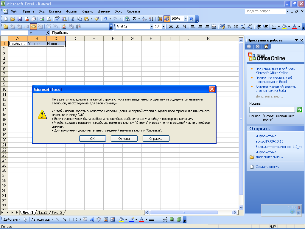


In this window, click the OK button. This will open the data entry form:


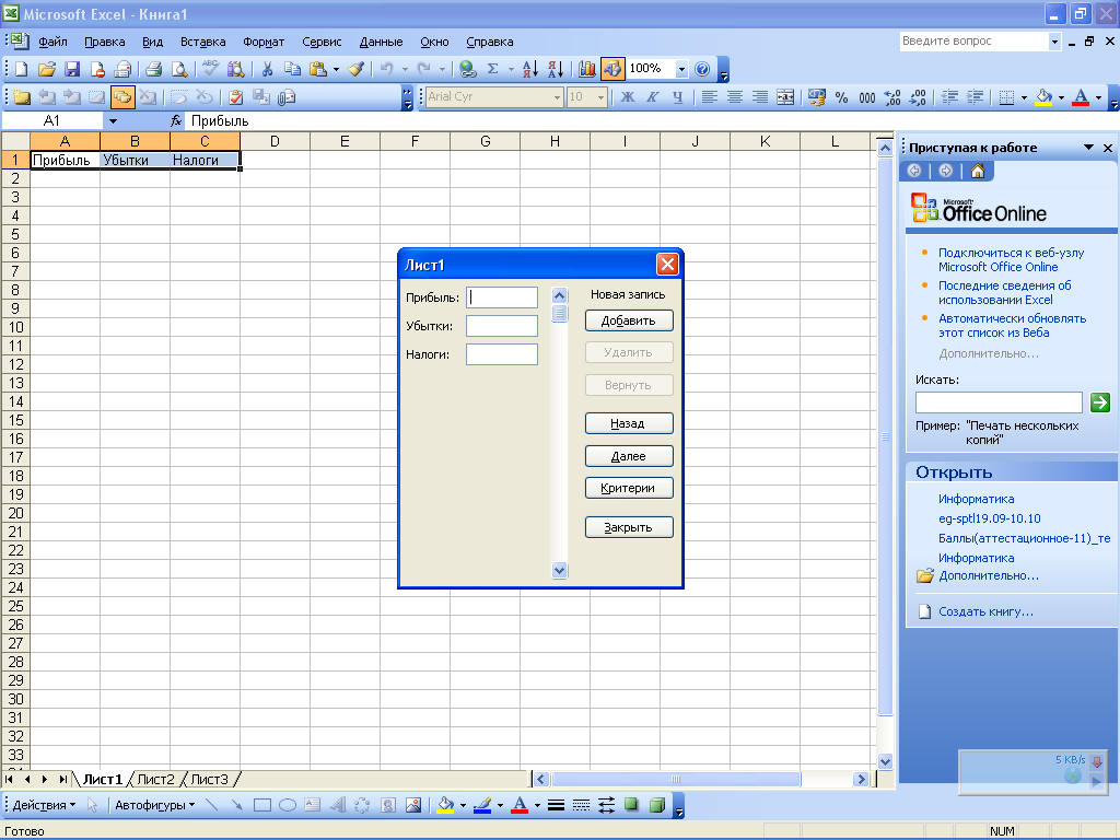
The figure shows that the fields located in the left part of this window are named according to the names of the columns of the table being filled. The procedure for entering data is as follows: in the fields Profit, Loss and Taxes, the necessary values ​​are entered, after which the button is pressed Add. As a result, the first row of the table will be filled in, and the fields will be cleared for entering data for the next row, and so on. If you need to return to the value entered in the table earlier, use the button Back. The button is used to move to the next values. Further. After entering all the necessary data into the table, click the button close. Similarly, you can fill in any tables, the volume of which is limited only by the size of the worksheet.

3.7 Drawing tables

As you know, an Excel worksheet is a table consisting of cells, each of which is located at the intersection of a row and a column. However, in most cases, it is required to design a visual representation of a particular table (or several tables) on a worksheet. In particular, you need to assign understandable names to rows and columns that briefly reflect their essence, define table boundaries, and so on. To create such tables, the program implements a special mechanism, which is accessed by the toolbar Border. IN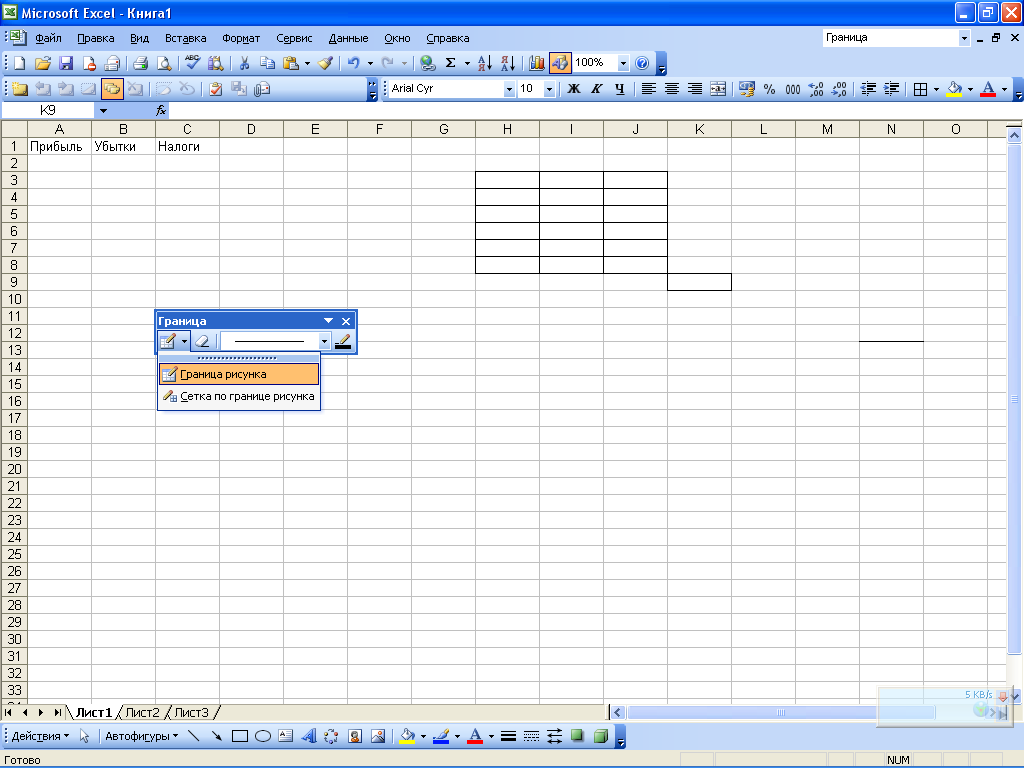

First of all, you should decide on what borders you need to draw. For example, the overall table border can be made thick, while the table grid can be made normal. To create a common border, you need to click the button located on the left of the toolbar, and in the menu that opens: select the item picture border. Then, with the mouse button pressed, the pointer (which will take the form of a pencil) should outline the border of the table. In order for each cell to be separated from one another by a border, you need to select the item in the menu of the first button of the Border panel. Pattern Border Grid, and then also outline the required range. The type and thickness of the border line is selected from the drop-down list. Here you can find the following types of lines: dotted, dash-dotted, double, etc. TO

You can assign a different color to each border line, if necessary. To select a color, click the button located on the right side of the toolbar. Line color(the name of this button is displayed as a tooltip when you move the mouse pointer over it) and in the menu that opens, click to select suitable color. In this case, a sample of the selected color will be displayed on this button. It should be noted that table borders are not deleted according to the usual rules, that is, using the Delete key. To remove the border, you need on the toolbar Border press the button Erase the border, then perform the same actions as when drawing a table (that is, with the mouse button pressed, you need to specify the lines that should be erased). To delete a line within one cell, just move the pointer to this line, which, after pressing the button Erase c Anitsu will take the form of an eraser, and click the mouse button.

3.8 Calculation of subtotals

When working with tables, it is often necessary to summarize intermediate results (for example, in a table with data for the year, it is advisable to calculate quarterly intermediate results). This can be done, for example, using the regular formula mechanism. However, this option may turn out to be quite cumbersome and not very convenient, because for this you need to perform a number of actions: insert new rows (columns) into the table, write the necessary formulas, etc. Therefore, to calculate subtotals, it is advisable to use a specially designed mechanism that is implemented in Excel. In order for the calculation of subtotals using this mechanism to be possible, the following conditions must be met: the first row of the table must contain the names of the columns, and the remaining rows must contain data of the same type. In addition, the table must not contain empty rows and columns. First of all, you need to select the table with which to work. Then you should switch to the mode of setting subtotals - this is the main menu command Data Results. When executed, a dialog box opens. Subtotals.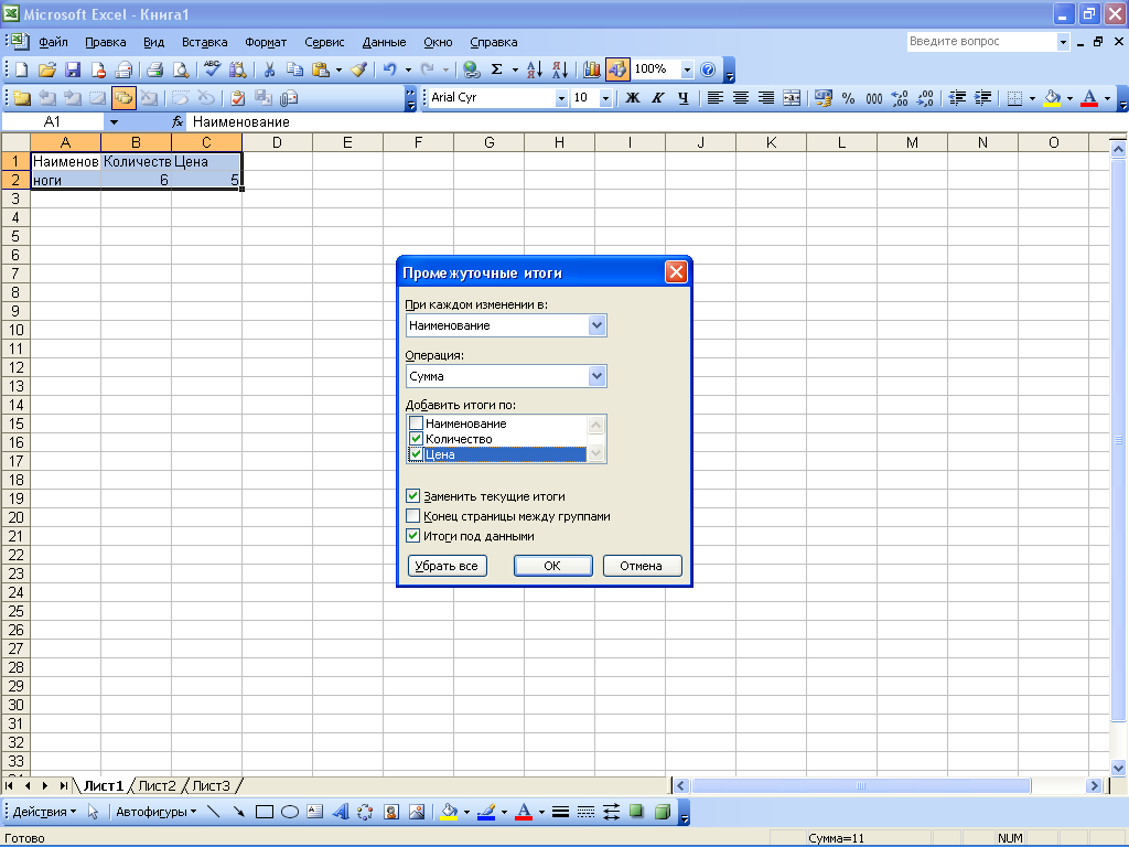


This window defines the values ​​of the parameters listed below.

With every change in- from this drop-down list (it includes the names of all columns of the table), you need to select the name of the table column, based on the data of which a conclusion will be made about the need to add a row of subtotals. To make it clear how the value of this field is processed, consider an example. Let's say the desired column is called Name of product, the first three positions in it are occupied by the product Trousers, the next four Shoes and two more - Mikey(all items of the same type differ only in price). If in the calculation window in the field With every change in select value Name of product, then rows with total data will be added to the table separately for all trousers, shoes and T-shirts. Operation– here, from the drop-down list, the type of operation that should be applied to calculate the subtotals is selected. For example, you can calculate the sum, product, display the arithmetic mean, find the minimum or maximum value, etc. Add totals for– in this field, by setting the appropriate checkboxes, you should define the columns of the table by which subtotals should be calculated. For example, if in our example the composition of the table in addition to the column Name of product more columns included Quantity And Price(the names of these flags are similar to the names of the columns of the table), since the calculation of intermediate (and general) totals for the column Name of product doesn't make sense . Replace Current Totals– this checkbox should be set if it is necessary to replace existing subtotals with new ones. This checkbox is checked by default. End of page between groups- when this box is checked, a page break will be automatically inserted after each subtotal line. By default, this checkbox is unchecked. Totals under the data– if this checkbox is checked, then the total rows will be located under the corresponding groups of positions, and if it is cleared, then above them. This checkbox is checked by default! Remove all– when this button is pressed, all existing rows with subtotals will be deleted from the table with simultaneous closing of the window Subtotals.

Push button OK the process of setting up the calculation of subtotals is completed. Button Cancel is designed to exit this mode without performing the calculation.

The main advantage of the editor of electronic Excel tables is the presence of a powerful apparatus of formulas and functions. Any data processing in Excel is carried out using this device. You can add, multiply, divide numbers, take square roots, calculate sines and cosines, logarithms and exponents.

Formula concept in Excel

A formula in Excel is a sequence of characters that starts with an equals sign "=". This sequence of characters can include constant values, cell references, names, functions, or operators.

The concept of a function in Excel

Functions in Excel are used to perform standard calculations in workbooks. The values ​​that are used to evaluate functions are called arguments. | The values ​​returned by functions as a response are called results.

Syntax rules for writing functions

If a function appears at the very beginning of a formula, it must be preceded by an equals sign, as is usual at the beginning of a formula. | Function arguments are written in parentheses immediately after the function name and are separated from each other by a semicolon ";".

Entering and editing formulas

In formulas, you can use addition "+", subtraction "-", multiplication "*", division "/", exponentiation "^". You can also use the percent sign "%", brackets "(", ")". When writing time, the colon character ":" is used.

Use of links

A link uniquely identifies a cell or group of cells in a worksheet. Links indicate which cells contain the values ​​that you want to apply as formula arguments. Using links, you can use data in different places in the worksheet in the formula, as well as use the value of the same cell in several formulas.

Using Names in Formulas

A name is an easy-to-remember identifier that can be used to refer to a cell, group of cells, value, or formula. The use of names provides the following benefits. | Formulas that use names are easier to read and remember than formulas that use cell references.

Error values ​​in formulas

Excel displays an error value in a cell when the formula for that cell cannot be calculated correctly. If a formula contains a cell reference that contains an error value, then that formula will also output an error value (unless you use the special functions of the worksheets ISERR, ISERROR, or YEND that check for error values).

Moving and copying formulas

After the formula is entered into a cell, you can move it, copy it, or distribute it to a block of cells. | When you move a formula to a new place in the table, the links in the formula do not change, and the cell where the formula used to be becomes free.

financial functions

Among the functions available in Excel, the section on financial transactions occupies a significant place. With its functions, you can perform calculations related to interest rates, securities, depreciation, payments, deposits, and more. | Table 4.5.

Date and time functions

The date and time representation has one peculiarity. When entering a date or time, you enter a sequence of characters that is not a number, but you can perform calculations with these characters: compare, add, subtract.

Math functions

Excel has a wide range of mathematical functions that allow you to perform actions from various areas of mathematics: arithmetic, algebra, combinatorics, etc. (see Table 4.8). | Table 4.8. Math functions. | ABS | Returns the modulus (absolute value) of a number. | ACOS

Statistical functions

In Excel, the most widely represented functions are designed to carry out various kinds of statistical calculations: the maximum and minimum values ​​of the range, probability values, distributions of random variables, averages, variances, confidence intervals, etc. | Table 4.9.

Functions for Working with References and Arrays

Excel has a number of functions for handling links and arrays: calculating the row or column numbers of a table from the name of the link, determining the number of columns (rows) of the link or array, selecting a value from the index number, and so on. | Table 4.10. Functions for working with links and arrays. | ADDRESS

Database Functions

Among Excel functions There is a section on database processing that allows you to do the following: Find the maximum and minimum values ​​in a range when you run a certain criterion, summing or multiplying numbers from a range, counting the number of nonblank cells, etc.

Text functions

In Excel, you can create formulas that allow you to perform various actions for processing text information: determining the number of characters in a string, extracting a substring from a string, converting text to a numeric value, changing case, and so on. | Table 4.12. Text functions. | DLSTR

Logic functions

Boolean functions are an essential component of many formulas. Whenever you need to perform certain actions depending on the fulfillment of any conditions, you use logical functions.

Functions for checking properties and values

In order to perform various kinds of checks in Excel, the functions of the Checking properties and values ​​section are used, which allow you to determine the type of value, display information about the current operating system, determine the type of error that occurred, etc. | Table 4.13. Functions for checking properties and values.

Statistical data analysis

Excel allows you to collect, process and interpret data, that is, to conduct statistical research. Statistics give you a condensed and concentrated view of your data. If we talk about the results of observations, then this is primarily the average value, the deviation from the average, the most probable value, the degree of reliability. All this applies to descriptive statistics.

Filtering data in a list

In Excel, a list is a labeled sequence of worksheet rows that contain the same type of data in the same columns. | List filtering allows you to find and select for processing some of the records in the list, table, database.

Work in the field of management and marketing is impossible to imagine without creating spreadsheets in Excel. Knowledge of this program is a basic skill for any employee whose responsibilities include analytics, forecasting, reporting, and presenting numerical data in a format that is convenient for work. If you are still unfamiliar with formulas in Excel, then here is a small instruction with which you can start mastering this program.

MATHEMATICAL (ARITHMETIC) OPERATORS

Excel uses standard operators for formulas, such as: sign plus for addition (+), minus for subtraction (-), star for multiplication (*), slash for division (/) and circumflex for exponentiation (^). 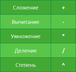All formulas in Excel must begin with an equal sign (=). This is because Excel equates the data stored in a cell (i.e. the formula) to the value it calculates (i.e. the result).

BASIC INFORMATION ABOUT LINKS

Although you can create formulas in Excel using fixed values ​​(for example, =2+2 or =5*5), in most cases cell addresses are used to create formulas. This process is called link building. When creating cell references, make sure that formulas do not contain errors. Using links in formulas provides a number of benefits, ranging from fewer errors to easier editing of formulas. For example, you can easily change the values ​​referenced in a formula without having to edit it.

Using mathematical operators, together with cell references, you can create a set simple formulas. The figure below shows some examples of formulas that use various combinations of operators and references.

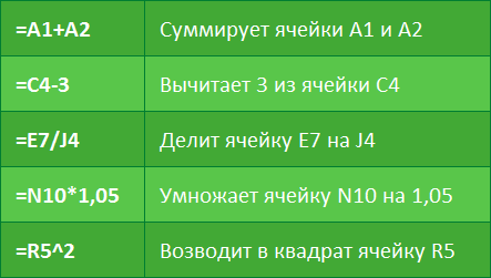
CREATING THE FIRST SIMPLE FORMULA IN EXCEL

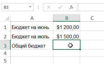
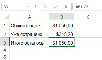
In the following example, we will calculate a simple budget for two months, for this we will create a simple formula with cell references.

1. To create a formula, select the cell that will contain it. In our example, we have selected cell B3.

2. Type an equal sign (=). Note that it appears both in the cell itself and in the formula bar.

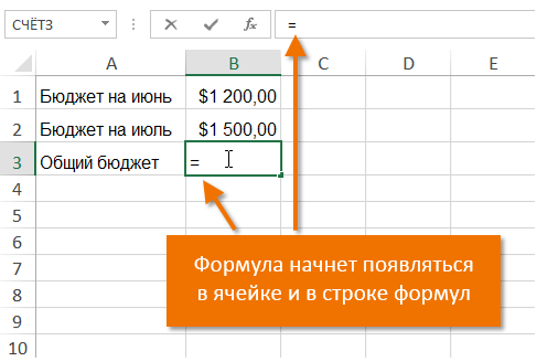3. Enter the address of the cell that should be the first in the formula. In our case, this is cell B1. Its borders will be highlighted in blue. 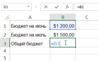4. Enter the math operator you want to use. In our example, we will enter the addition sign (+). 5. Enter the address of the cell that should be the second in the formula. In our case, this is cell B2. Its borders will be highlighted in blue. 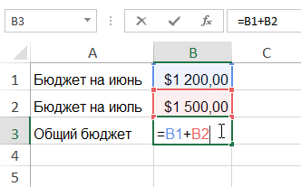6. Click Enter

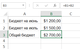
THE MAIN ADVANTAGE OF FORMULA WITH REFERENCES

The main advantage of links is that they allow you to make changes to the data in an Excel worksheet without having to rewrite the formulas themselves. In the following example, we will change the value of cell B1 from $1200 to $1800. The formula will be automatically recalculated and the new value will be displayed.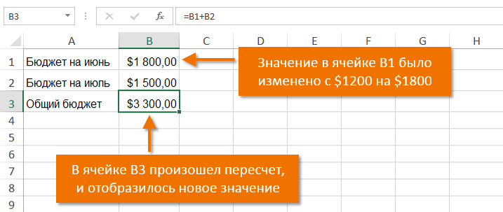

CREATING A FORMULA IN EXCEL BY SELECTING A CELL WITH THE MOUSE

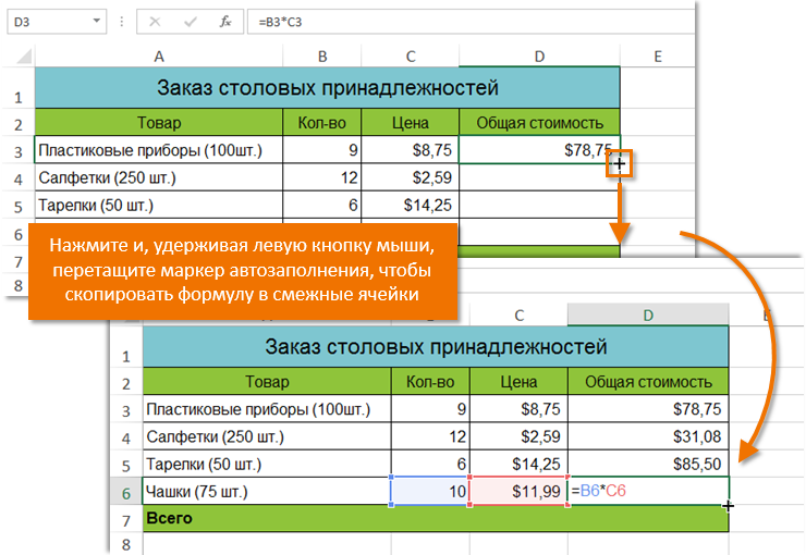
Instead of entering cell addresses manually, you can simply click on the cell you want to include in the formula. This trick can save you a lot of time and effort when creating formulas in Excel. In the following example, we will create a formula to calculate the cost of ordering multiple boxes of plastic tableware.

1. Select the cell that will contain the formula. In our example, we have selected cell D3.

2. Type an equal sign (=). 3. Select the cell that should be the first in the formula. In our case, this is cell B3. The cell address will appear in the formula, with a blue dotted line around it.

4. Enter the math operator you want to use. In our example, this is the multiplication sign (*). 5. Select the cell that should be the second in the formula. In our case, this is cell C3. The cell address will appear in the formula, with a red dotted line around it.

6. Click Enter on keyboard. The formula will be created and calculated.

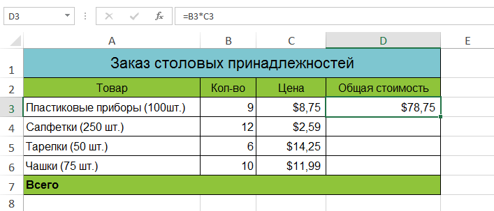
Formulas can be copied to adjacent cells using the autocomplete token. This will save time when you need to use the same formula many times. Check out the lessons in Relative and Absolute Links for more information.

HOW TO CHANGE FORMULA IN EXCEL

In the example below, we entered the wrong cell reference in the formula and we need to fix it.

1. Select the cell in which you want to change the formula. In our example, we have selected cell B3.

2. Click the Formula Bar to start editing the formula. You can also double-click a cell to view and edit the formula right there.

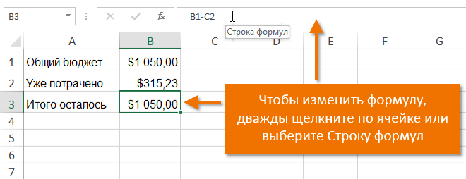3. All cells referenced by the formula will be highlighted with colored borders. In our example, we'll change the second part of the formula to point to cell B2 instead of C2. To do this, select the address you want to edit in the formula, and then select the required cell with the mouse or change the address manually.

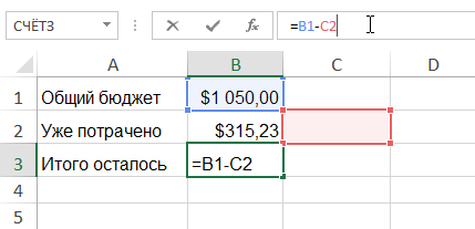4. When finished, press Enter on the keyboard or use the command Input in the formula bar. 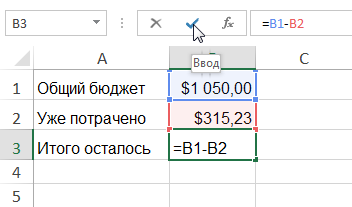5. The formula will update and you will see the new value. If you change your mind, you can press the key Ess on the keyboard or click command Cancel in the Formula Bar to avoid accidental changes.

PROCEDURE IN EXCEL FORMULA

Excel performs actions based on the following order:

1. Expressions enclosed in parentheses.
2. Exponentiation (for example, 3 2).
3. Multiplication and division, whichever comes first.
4. Addition and subtraction, which comes first.

EXAMPLE OF SOLVING A COMPLEX FORMULA

As an example, let's try to calculate the value of the formula shown in the following figure. At first glance, this expression looks rather complicated, but we can use the order of operations in stages to find the correct answer. 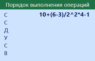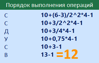You will get exactly the same result if you enter this formula in Excel.

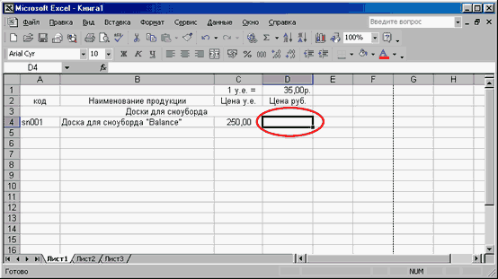
Finally, we have come to the implementation of one of the features of the program "Excel" - working with calculation formulas. Cell "D4" should contain the result of multiplying the price of the goods in c.u. (cell "C4") and today's rate (cell "D1"). How to do it? We mark the cell where the result should be located by clicking the left mouse button.

To create a formula, left-click on the arrow next to the "AutoSum" button on the toolbar and select "More Functions...". Or go to the "Insert" menu and select "Function".

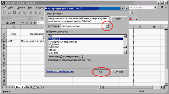
A window opens to help you enter the formula. From the "Category" list, select the "Math" item. (Please note that in fact the program can work with various categories of functions. These are financial, and statistical, and working with data, and much more). In the list of functions we find "PRODUCTION". After that, click on the "OK" button.

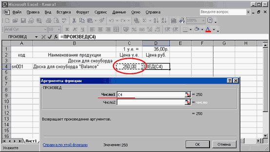
First, we are asked to specify the cell from which the data for the first multiplier should be taken. Enter the designation of the desired cell - "C4".

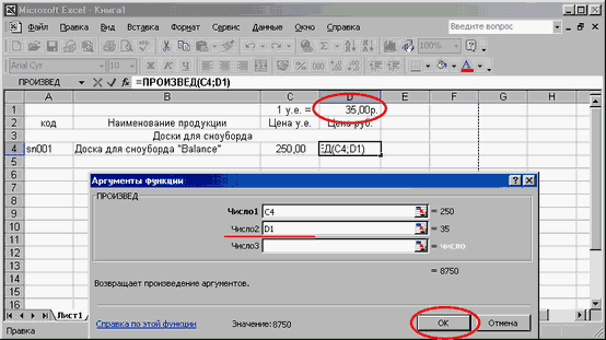
Next step: the cell where the second multiplier is located - "D1". Of course, a specific number that we enter directly into the field can also act as data. On the right we control the result. After entering the data, click on the "OK" button.

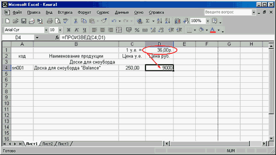
In cell "D4" we see the finished result. Now we need to change the exchange rate data of a conventional unit - and the program will do the recalculation itself. Comfortable? Certainly!