The SUMIF function is used when you want to sum the values in a range that meet a specified criterion.
Function Description
The SUMIF function is used when you want to sum the values in a range that meet a specified criterion. For example, in a column of numbers, you want to sum only values greater than 5. You can use the following formula to do this:
=SUMIF(B2:B25,">5") this example summed values are checked for compliance with the criterion. If necessary, the condition can be applied to one range, and sum the corresponding values from another range. For example, the formula:
=SUMIF(B2:B5, "Jan", C2:C5) sums only those values in the range C2:C5 for which the corresponding values in the range B2:B5 are "Jan".
Another example of using the function is shown in the figure below:
An example of using SUMIF to calculate profit with a condition
Syntax
=SUMIF(range, condition, [sum_range])Arguments
range condition sum_range
Required argument. The range of cells that are evaluated against the criteria. The cells in each range must contain numbers, names, arrays, or references to numbers. Empty cells and cells containing text values are skipped.
Required argument. A condition in the form of a number, expression, cell reference, text, or function that determines which cells to sum. For example, a condition can be represented as: 32, “>32”, B5, “32”, “apples”, or TODAY().
Important! All text conditions and conditions with logical and mathematical signs must be enclosed in double quotes (“). If the condition is a number, you do not need to use quotation marks.
Optional argument. Cells whose values are summed if they differ from the cells specified as a range. If the sum_range argument is omitted, Microsoft Excel sums the cells specified in the range argument (the same cells that the condition applies to).
Remarks
- You can use wildcards in the condition argument: question mark (?) and asterisk (*). A question mark matches any single character, and an asterisk matches any sequence of characters. If you want to search directly for a question mark (or an asterisk), you must precede it with a tilde (~).
- The SUMIF function returns incorrect results when it is used to match strings longer than 255 characters against #VALUE!.
- The sum_range argument may not be the same size as the range argument. When determining the actual cells to be summed, the top-left cell of the sum_range argument is used as the starting cell, and then the cells of the portion of the range that matches the size of the range argument are summed.
SUMIF function. The first of three Excel whales
I begin the review of the main tools of our favorite program from Microsoft. And of course, at the beginning I want to talk about my most frequently used function (“formula”). More specifically, the SUMMESLI function. If you have no idea what it is and how to use it - I envy you! For me it was a real discovery.
Did you have to sum up data on employees or clients from a large table, choose how much revenue was for one or another nomenclature? Did you filter by last name/position and then enter the numbers by hand into separate cells? Maybe on a calculator? What if there are more than a thousand rows? How to calculate quickly?
This is where SUMMESLI comes in handy!
Task1. There are statistics on goods, cities and what indicators were achieved for these positions. It is necessary to calculate:How much was the product item 1 sold for?
Before proceeding to the solution of the 1st problem, let's analyze what the SUMIF function consists of:
- Range. The range that contains the search terms. Required to fill out. For the 1st task, the Product column.
- Criterion. Can be filled with a number (85), an expression (">85"), a cell reference (B1), a function (today()). Defines the condition by which summed (!). All text conditions are enclosed in quotation marks ( « ) ">85". Required to fill out. For the 1st task column =Product1
- Sum_range. Cells to sum if they are different from the cells in the Range. For the 1st task, the Revenue column.
So let's write the formula, having previously entered the condition argument in cell F3

Don't forget to check Did it count? Right? Great!
Those. selection must be made on two parameters. To do this, use the SUMIF function for several conditions - SUMIFS, where the recording order and the number of arguments are slightly changed.


And also to count the number of repetitions of a particular position, use the functions COUNTIF (COUNTIFS)
It is even easier to solve than the previous two.

Part 2
What is SUMMESLI?
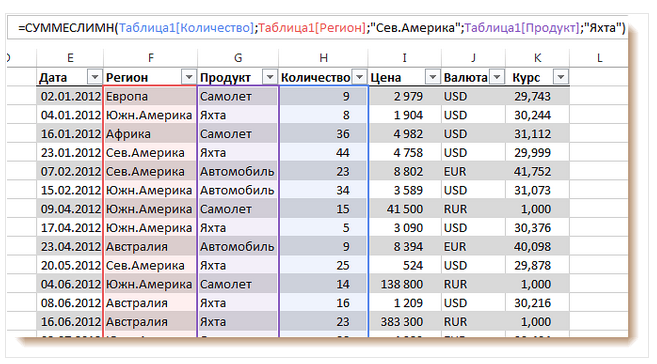
Probably everyone who works quite often in Excel knows about the existence of such a function as SUMIF, which allows you to sum only those values from a data set that satisfy some alone condition. I have already given an example of data that can be analyzed in this way:
Suppose you need to find the number of yachts sold. In this case, you can use one of the formulas:
=SUMIF(Table 1 [Product]; "Yacht" ;Table 1 [Number]) =SUMIF(C2 : C40 ; "Yacht" ; D2 : D40 )Problem
However, with a more complex analysis, the SUMIF function will not cope for a very obvious reason - it selects data only one by one condition. No options. So, for example, if you want to know how many yachts were sold in North America, then the SUMIF function will not help you.
However, there are at least three alternatives:
- Use array formulas to summarize data by multiple criteria.
- Use the SUMPRODUCT function
- Use the SUMIFS function
There is, however, another solution for which even Excel is not needed - to go to North America and count the yachts, but this, fortunately, is not our method!
Solution
So, let's use the third of the proposed solutions and write down the following formula:
=SUMIFS(Table 1 [Quantity];Table 1 [Region]; "North America" ;Table 1 [Product]; "Yacht")Pay attention to how the data ranges and arguments of this function correspond:
How does SUMIFS work?
Everything is simple here. The SUMIFS function requires you to specify the range of cells that contain the numbers to be summed, as well as at least one cell range-selection criteria pair. You can specify up to 127 such pairs, which allows you to analyze all conceivable combinations of conditions and criteria.
To better remember the order of the arguments to this function, look at the figure:
Bonus
And not one, but two!
First, in Excel 2007 and later, there is a small family of similar functions, including AVERAGEIFS (for calculating averages) and COUNTIFS (for counting the number of values).
Secondly, the functions of this family can work with relational operators (>,<, = и т.п.) и знаками подстановки, такими как «*» — любое количество любых символов, и «?» — один любой символ. Так, например, чтобы подсчитать количество самолетов, проданных в Северной и Южной Америке, можно воспользоваться такой формулой:
=SUMIFS(Table 1 [Quantity];Table 1 [Region]; "*America" ;Table 1 [Product]; "Airplane" )Let's add the values located in the rows, the fields of which satisfy two criteria at once (Condition AND). Consider Text Criteria, Numeric Criteria, and Date Criteria. Let's analyze the function SUMIFS( ) , the English version of SUMIFS().
As a source table, let's take a table with two columns (fields): text " Fruits" and numerical " Quantity in stock» (See example file).
Task1 (1 text criterion and 1 numerical criterion)
Let's find the number of boxes of goods with a certain fruit AND, which Remaining boxes in stock not less than the minimum. For example, the number of boxes with goods peaches ( cell D 2 ), who have a balance of boxes in stock >=6 ( cell E 2 ) . We should get the result 64. The calculation can be implemented with a variety of formulas, here are a few (see the example file Sheet Text and Number):
1. =SUMIFS(B2:B13;A2:A13;D2;B2:B13;">="&E2)
Function syntax: SUMIFS(summation_interval, condition_interval1, condition1, condition_interval2, condition2…)
- B2:B13 Sum_interval- cells for summation, including names, arrays or references containing numbers. Empty values and text are ignored.
- A2:A13 And B2:B13 Condition_interval1; condition_interval2; … are from 1 to 127 ranges in which the corresponding condition is checked.
- D2 And ">="&E2 Condition1; condition2; … are from 1 to 127 conditions in the form of a number, expression, cell reference, or text that determine which cells will be summed.

The order of the arguments is different in the SUMIFS() and SUMIFS() functions. The SUMIFS() argument sum_interval is the first argument, and in SUMIF() it is the third. When copying and editing these similar functions, care must be taken to ensure that the arguments are specified in the correct order.
2. other option = SUMPRODUCT((A2:A13=D2)*(B2:B13);--(B2:B13>=E2))
Let's take a closer look at using the SUMPRODUCT() function:
- The result of A2:A13=D2 is an array (FALSE:FALSE:FALSE:FALSE:TRUE:TRUE:TRUE:FALSE:FALSE:FALSE:FALSE:FALSE) A criterion, i.e. word peaches. The array can be seen by highlighting in A2:A13=D2 and then pressing ;
- The result of calculating B2:B13 is (3:5:11:98:4:8:56:2:4:6:10:11), i.e. just values from a column B ;
- The result of element-wise multiplication of arrays (A2:A13=D2)*(B2:B13) is (0:0:0:0:4:8:56:0:0:0:0:0). Multiplying a number by FALSE results in 0; and on the value TRUE (=1) the number itself is obtained;
- Let's analyze the second condition: The result of calculation --(B2:B13>=E2) is an array (0:0:1:1:0:1:1:0:0:1:1:1). Values in column " Number of boxes in stock” that satisfy the criterion >=E2 (i.e. >=6) correspond to 1;
- Further, the SUMPRODUCT() function multiplies the array elements in pairs and sums the resulting products. We get - 64.
3. Another use case for the SUMPRODUCT() function is the formula =SUMPRODUCT((A2:A13=D2)*(B2:B13)*(B2:B13>=E2)).
If necessary, dates can be entered directly into the formula = SUMIFS(B6:B17;A6:A17;">=15.01.2010";A6:A17;"<=06.03.2010")
To display the selection criteria in a text line, use the formula ="Sales for the period from "&TEXT(D6;"dd.MM.yy")&" to "&TEXT(E6;"dd.MM.yy")
used in the last formula.
Task4 (Month)
We slightly modify the condition of the previous task: find the total sales for the month (see the example file Leaf Month).
Formulas are built similarly to task 3, but the user enters not 2 dates, but the name of the month (it is assumed that the data in the table is within 1 year).

To solve the 3rd task, the table with the configured autofilter looks like this (see the example file Sheet 2 Dates).

The table must first be converted to and include the Total row.
Good afternoon, dear subscribers and visitors of the blog site. Most recently, we figured out the VLOOKUP formula, and right after that, I decided to write about another very useful Excel function - SUMIF. Both of these functions are able to “link” data from different sources (tables) by key field and under certain conditions are interchangeable. At the same time, there are significant differences in their purpose and use.
If the purpose of the VLOOKUP is simply to “pull up” data from one place in Excel to another, then SUMIF is used to sum the numerical data according to a given criterion. The main purpose of this formula is to sum the data according to some condition. This is what it says in the manual. However, this tool is useful for other purposes as well. For example, I often use the SUMIF formula instead of VLOOKUP because it doesn't throw #N/A errors when it can't find something. This makes the job much easier and faster.
The SUMIF function can be successfully adapted to solve a wide variety of problems. Therefore, in this article we will consider not 1 (one), but as many as 2 (two) examples. The first will be associated with summation according to a given criterion, the second - with data "pulling up", that is, as an alternative to VLOOKUP.
Example of summing using the SUMIF function
The table shows the positions, their quantities, as well as belonging to a particular group of goods (first column). For now, let's consider the simplified use of SUMIF, when we need to calculate the sum only for those positions, the values for which meet a certain condition. For example, we want to know how many top positions were sold, i.e. those whose value exceeds 70 units. It is not very convenient and fast to search for such goods with your eyes, and then sum it up manually, so the SUMIF function is very appropriate here.
First of all, select the cell where the amount will be calculated. Next, we call the Function Wizard. This is an icon fx in the formula bar. Next, look for the SUMIF function in the list and click on it. A dialog box opens where, to solve a particular task, you need to fill in only two (first) fields out of three proposed.

That's why I called this example simplified. Why 2 (two) out of 3 (three)? Because our criterion is in the summation range itself.
The "Range" field indicates the area of the Excel table where all the original values \u200b\u200bare located, from which something needs to be selected and then added. It is usually set with the mouse.
The Criteria field specifies the condition by which the formula will select. In our case, we indicate "> 70". If you do not put quotes, then they will be drawn on their own. But in general, such a criterion should be in quotation marks.
The last field "Summation_range" is not filled in, since it is already indicated in the first field.
Thus, the SUMIF function takes a criterion and begins to select all values from the specified range that satisfy the given criterion. After that, all the selected values are added up. This is how the function algorithm works.
Having filled in the required fields in the Functions Wizard, press the large “Enter” button on the keyboard, or click on “OK” in the Wizard window. After this action, the calculated value should appear in place of the introduced function. In my example, it turned out 224 pieces. That is, the total value of goods sold in the amount of more than 70 pieces was 224 pieces. (this can be seen in the lower left corner of the Wizard window even before clicking "ok"). That's all. This was a simplified example where the criterion and summation range are in the same place.
Now let's look at an example where the criterion does not match the summation range. This situation is much more common. Consider the same conditional data. Suppose we need to find out the amount no more or less than some value, and the amount of a specific group of goods, for example, group G.
To do this, select the cell with the future calculation of the sum again and call the Function Wizard. Now in the first window we indicate the range, which contains the criterion by which the selection will be made for summation, that is, in our case, this is a column with the names of product groups. Next, the criterion itself is written either manually, leaving the entry “G group” in the corresponding field, or simply pointing the cell with the desired criterion with the mouse. The last box is the range where the summarized data is located. We indicate it with the mouse, but print lovers are not forbidden to type it manually.

The result will be the sum of goods sold from group G - 153 pieces.
So, we have looked at how to calculate one sum by one specific criterion. However, more often a problem arises when it is required to calculate several amounts for several criteria. There is nothing easier! For example, we need to find out the amount of goods sold for each group. That is, 4 (four) values are of interest for 4 (four) groups (A, B, C and D). To do this, usually somewhere in the expanses of Excel a list of groups is made in the form of a separate plate. It is clear that the names of the groups must exactly match the names of the groups in the source table. Immediately add the final line, where the sum is still zero.

Then the formula for the first group is written and extended to all the others. Here only it is necessary to pay attention to the relativity of references. The range with the criteria and the summation range must be absolute references so that when the formula is dragged, they do not “go down”, but the criterion itself, firstly, you need to specify with the mouse (and not type it manually), and secondly, it must be a relative reference, so how each sum has its own summation criterion.
The filled fields of the Function Wizard in such a calculation will look something like this.

As you can see, for the first group A, the amount of goods sold was 161 pieces (lower left corner of the figure). Now press enter and drag the formula down.

All amounts have been calculated, and their total is 535, which is the same as the total in the original data. So, all the values were summed up, nothing was missed. The last use case for SUMMESLI is quite common for me personally.
Example of using the SUMIF function to match data
As I have pointed out more than once, the SUMIF function can be usefully used for data binding. Indeed, if you sum up one value, you get this value itself. This arithmetic property is not a sin to use for good. It is even possible that the designers of Excel are not aware of such a barbaric use of their offspring.
In short, SUMIF is easy to adapt for databinding as an alternative to the VLOOKUP function. Why use SUMIF if there is a VLOOKUP? I explain. First, SUMMIF, unlike VLOOKUP, is insensitive to the data format and does not throw an error where you least expect it; secondly, instead of errors due to the lack of values for a given criterion, SUMMIF gives 0 (zero), which allows you to calculate the totals of the range with the SUMMESLI formula without unnecessary gestures. However, there is one downside. If any criterion is repeated in the required table, then the corresponding values will be summed up, which is not always a “pull-up”. Better be on your guard. On the other hand, this is often what is needed - to pull up the values to a given place, and add the duplicated positions at the same time. You just need to know the properties of the SUMIF function and use it according to the instruction manual.
Now let's look at an example of how the SUMIF function is more suitable for data pull-up than VLOOKUP. Let the data from your example be the sales of some goods for January. We want to know how they changed in February. It is convenient to make a comparison in the same table, after adding one more column to the right and filling it with data for February. Somewhere in another Excel file there are statistics for February for the entire range, but we want to analyze these particular positions, for which we need to pull the necessary values into our table from a large file with sales statistics for all products. First, let's try to use the VLOOKUP formula. As a criterion, we will use the product code. The result is in the picture.

It is clearly seen that one position was not pulled up, and instead of a numerical value, the #N/A error is returned. Most likely, this product was simply not sold in February and therefore it is not in the database for February. As a consequence, the #N/A error is also shown in the total. If there are not many positions, then the problem is not big, it is enough to manually remove the error and the amount will be correctly recalculated. However, the number of lines can be measured in hundreds, and counting on manual adjustment is not quite the right decision. Now let's use the SUMIF formula instead of VLOOKUP.

The result is the same, but instead of the #N/A SUMMIF error, it returns zero, which allows you to normally calculate the sum (or other indicator, for example, the average) in the total row. This is the main idea why SUMIF should sometimes be used instead of VLOOKUP. With a large number of positions, the effect will be even more noticeable.
In reality, you often have to work with large amounts of data that are many times larger than the size of the monitor. It is very difficult to see and track errors. But all the shoals emerge in subsequent calculations. Such examples are not convenient to parse with the help of screenshots in the article, so I invite you to watch a specially recorded video tutorial about the SUMIF function.
And here is another lesson on SUMIF