When comparing several comparable objects in Excel tables, data is often organized into columns so that it is convenient to compare the characteristics of these objects row by row. For example, car models, telephones, experimental and control groups, a number of retail chain stores, etc. large numbers strings visual analysis may not be reliable. The functions VLOOKUP, INDEX, POISKPOZ (VLOOKUP, INDEX, MATCH) are convenient for comparing data across cells and do not give an overall picture. But how to find out how similar the columns are in general to each other? Are the columns identical?
The Map Columns add-on allows you to map columns and see the big picture:
- Compare two or more columns with each other
- Compare columns with reference values
- Calculate exact match percentage
- Present the result in a visual pivot table
Video language: English. Subtitles: Russian, English. (Note: Video may not reflect Latest updates. Use the instructions below.)
Add "Match Columns" in Excel 2016, 2013, 2010, 2007
Suitable for: Microsoft Excel 2016 - 2007, desktop Office 365 (32-bit and 64-bit).
How to work with the add-on:
How to compare two or more columns with each other and calculate the match percentage
Consider an example of product development. Suppose you need to compare several finished prototypes with each other and find out how similar, different and perhaps even identical they are.
- Click the "Map Columns" button in the XLTools panel > Select "Map Columns Together".
- Click OK >

Advice:
Select pivot table result > Click on the Express Analysis icon > Apply "Color Scale".
Reading the result: Type 1 and Type 3 prototypes are almost identical, with a 99% match rate indicating that 99% of their string parameters match. Type 2 and Type 4 are the least similar - their parameters match only 30%.
How to Compare Columns to Reference Values and Calculate the Match
Consider an example of product development. Suppose you need to compare several finished prototypes to a certain target standard, and also calculate the degree of conformity of the prototypes to these standards.
- Select columns to compare.
For example, columns with prototype data. - Click the Map Columns button in the XLTools panel.
- Select Map to Range of Reference Columns > Select Reference Columns.
For example, columns with standards. - Check "Columns contain headers" if so.
- Check "Show Percent Match" to display the match as a percentage.
Otherwise, the result will be displayed as 1 (full match) or 0 (no match). - Specify whether the result should be placed on a new sheet or on an existing sheet.
- Click OK > Done, the result is presented in the pivot table.

Advice: to make it easier to interpret the result, apply to it conditional formatting:
Select the summary table of the result > Click on the Express Analysis icon > Apply "Color Scale".
Result reading: Type 2 prototype is 99% compliant with Standard 2, i.e. 99% of their parameters in the lines are the same. Product 5 is closest to Standard 3 - 96% of their parameters are identical. At the same time, Product 4 is far from meeting any of the three standards. Now we can conclude how much each of the prototypes deviates from the target reference values.
What tasks can the Match Columns add-in help with?
The add-in scans the cells line by line and calculates the percentage of the same values in the columns. XLTools "Match Columns" is not suitable for general comparison of values in cells - it is not designed to find duplicates or unique values.
The Map Columns add-in has a different purpose. Its main task is to find out how, in general, data sets (columns) are similar or different. The add-on helps with the analysis of a large amount of data when you need to look wider, at a macro level, for example. answer questions like:
- How similar are the performance of the experimental groups
- How similar are the results of the experimental and control groups
- How similar / different are several products of the same category
- How close are KPI indicators of employees to planned indicators?
- How similar are the performance of several retail stores, etc.
If you are working with large spreadsheet documents (a lot of data/columns), it is very difficult to control the accuracy/relevance of all information. Therefore, it is very often necessary to analyze two or more columns in an Excel document to detect duplication. And if the user does not have information about all the functionality of the program, he may logically have a question: how to compare two columns in excel?
The answer has long been thought up by the developers of this program, who initially put in it commands that help compare information. In general, if you go into the depths of this issue, you can find about a dozen different ways, including writing individual macros and formulas. But practice shows: it is enough to know three or four reliable ways to cope with the emerging needs of comparison.
How to compare two columns in excel for matches
Data in Excel is usually compared between rows, between columns, with a value given as a benchmark. If there is a need to compare columns, you can use the built-in functionality, namely, the Match and If actions. And all you need is Excel not earlier than the seventh year of "release".
We start with the function "Coincidence". For example, the data being compared is in columns with addresses C3 and B3. The result of the comparison must be placed in a cell, for example, D3. We click on this cell, enter the "formulas" menu directory, find the line "library of functions", open the functions placed in the drop-down list, find the word "text" and click on "Coincidence".
In a moment you will see on the display new form, where there will be only two fields: "text one", "text two". You need to fill in them, just, the addresses of the compared columns (C3, B3), then click on the usual “OK” key. As a result, you will see the result with the words "True" / "False". In principle, nothing particularly complicated even for a novice user! But this is far from the only method. Let's break down the "If" function.
Ability to compare two columns in excel for matches using "If" allows you to enter values that will be displayed in the end after the operation. The cursor is placed in the cell where the input will be made, the menu directory "library of functions" opens, the line "logical" is selected in the drop-down list, and the first position in it will be occupied by the "If" command. We choose it.
Further the form of the reasoned filling takes off. "Logic_expression" is the formulation of the function itself. In our case, this is a comparison of two columns, so we enter "B3 \u003d C3" (or your column addresses). Further fields "value_if true", "value_if_false". Here you should enter the data (labels/words/numbers) that should correspond to a positive/negative result. After filling, click, as usual, "ok". Let's get acquainted with the result.
If you want to perform line-by-line analysis of two columns, in the third column we put any function that was discussed above (“if”, or “coincidence”). Its action is extended to the entire height of the filled columns. Next, select the third column, click the "main" tab, look for the word "styles" in the group that appears. The "column/cell selection rules" will open.
In them you need to select the “equals” command, then click on the first column and press “Enter”. As a result, it turns out to “tint” the columns where there are matching results. And you will immediately see the information you need. Further, in the analysis of the topic "how to compare the values of two columns in excel", let's move on to a method such as conditional formatting in Excel.
Excel: conditional formatting
Formatting a conditional type will allow you not only to compare two different columns/cells/lines, but also to highlight different data in them with a given color (red). That is, we are not looking for coincidences, but differences. To get it, we act like this. We select the necessary columns, without touching their names, go to the “main” menu directory, in it we look for the “styles” subsection.
It will contain the line "conditional formatting". By clicking on it, we get a list where we need the “create rule” function item. Next step: in the "format" line, you need to drive in the formula = $ A2<>$B2. This formula will help Excel understand what exactly we need, namely, to color in red all the values of column A that do not equal the values of column B. A slightly more complicated way to apply formulas relates to the participation of structures such as HLOOKUP / VLOOKUP. These formulas refer to horizontal/vertical value lookups. Let's consider this method in more detail.
HLOOKUP and VLOOKUP
These two formulas allow you to search for data horizontally/vertically. That is, H is horizontal, and V is vertical. If the data to be compared is in the left column relative to the one where the compared values are located, use the VLOOKUP construct. But if the data for comparison is horizontally at the top of the table from the column where the reference values are indicated, we use the HLOOKUP construction.
To understand how to compare data in two excel columns vertically, the following full formula should be used: lookup_value,table_array,col_index_num,range_lookup.
The value to be found is denoted as "lookup_value". The search columns are driven in like a "table array". The column number should be specified as "sol_index_num". Moreover, this is the column, the value of which coincided, and which needs to be returned/corrected. The "range lookup" command here acts as an additional one. It can indicate whether the value needs to be made exact or approximate.
If this command is not specified, values will be returned for both types. The HLOOKUP formula looks like this in full: lookup_value,table_array,row_index_num,range_lookup. Working with it is almost identical to the one described above. True, there is an exception here. This is the index of the string, specifying the string whose values are to be returned. If you learn to clearly apply all of the above methods, it becomes clear: there is no more convenient and universal program for working with large quantity data different types than Excel. Comparing two columns in excel is, however, only half the job. After all, something else needs to be done with the obtained values. That is, the found matches still need to be processed somehow.
How to Handle Duplicate Values
So, there are numbers found in the first, suppose, column, completely repeating in the second column. It is clear that manually correcting repetitions is unrealistic work, taking up a lot of precious time. Therefore, you should use a ready-made technique for automatic correction.
For this to work, you must first name the columns if they don't exist. We adjust the cursor to the first line, right-click, in the menu that appears, select "insert". Let's say the headers are "name" and "duplicate". Next, you need the "date" directory, in it - "filter". Click on the tiny arrow next to the "duplicate" and remove all the "birds" from the list. Now click OK, and the duplicate values of column A become visible.
Next, we select these cells, because we needed not only to compare the text in two columns in excel, but also to remove duplicates. Selected, right-clicked, selected "delete row", clicked "ok" and got a table without matching values. The method works if the columns are on the same page, that is, they are adjacent.
Thus, we have analyzed several ways to compare two columns in Excel. I deliberately did not show you screenshots, because you would get confused in them.
BUT I have prepared a great video of one of the most popular and simple ways comparing two columns in the document and now I suggest you familiarize yourself with it in order to consolidate the material covered.
If the article was still useful for you, then share it on social media. networks or rate by clicking on the number of stars that you see fit. Thank you, that's all for today, see you soon.
© Alexander Ivanov.
Often the task is to compare two lists of elements. Doing it manually is too tedious, and besides, the possibility of errors cannot be ruled out. Excel makes this operation easy. This tip describes a method using conditional formatting.
On fig. 164.1 is an example of two multi-column lists of names. Applying conditional formatting can make differences in lists more obvious. These examples of lists contain text, but this method also works with numeric data.
The first list is A2:B31, this range is called old list. The second list is D2:E31 , the range is called new list. The ranges were named with the command Formulas Defined names Assign a name. Naming the ranges is optional, but it makes them easier to work with.
Let's start by adding conditional formatting to the old list.
- Select range cells old list.
- Select .
- In the window Create a formatting rule select the item named Use Formula
- Enter this formula in the window field (Fig. 164.2): =COUNTIF(NewList;A2)=0 .
- Click the button Format and set the formatting to be applied when the condition is true. It is best to choose different fill colors.
- Click OK.

Cells in a range new list use a similar conditional formatting formula.
- Select range cells new list.
- Select Home Conditional Formatting Create Rule to open a dialog box Create a formatting rule.
- In the window Create a rule formatting select item Use Formula to define the cells to be formatted.
- Enter this formula in the window box: =COUNTIF(OldList;D2)=0 .
- Click the button Format and set the formatting that will be applied when the condition is true (different fill color).
- Click OK.
As a result, the names that are in the old list, but which are not in the new one, will be highlighted (Fig. 164.3). In addition, names in the new list that are not in the old list are also highlighted, but in a different color. Names that appear in both lists are not highlighted.
Both conditional formatting formulas use the function COUNTIF. It counts how many times a certain value appears in a range. If the formula returns 0, it means the element is not in the range. So the conditional formatting takes over and the background color of the cell changes.

This is a chapter from a book: Michael Girvin. Ctrl+Shift+Enter. Mastering array formulas in Excel.
Selections based on one or more conditions. Row Excel functions use comparison operators. For example, SUMIF, SUMIFS, COUNTIF, COUNTIFS, AVERAGEIF, and AVERAGEIFS. These functions make selections based on one or more conditions (criteria). The problem is that these functions can only add, count, and average. And if you want to impose conditions on the search, for example, the maximum value or standard deviation? In these cases, since there is no built-in function, you must invent an array formula. Often this is due to the use of the array comparison operator. The first example in this chapter shows how to calculate the minimum value under one condition.
Let's use the IF function to select the elements of an array that meet a condition. On fig. 4.1 in the left table there is a column with the names of cities and a column with time. It is required to find the minimum time for each city and place this value in the corresponding cell of the right table. The selection condition is the name of the city. If you use the MIN function, you can find the minimum value of column B. But how do you select only those numbers that apply only to Auckland? And how do you copy the formulas down the column? Since Excel does not have a built-in MINESLI function, you need to write an original formula that combines the IF and MIN functions.
Rice. 4.1. Purpose of the formula: to select the minimum time for each city
Download note in format or in format
As shown in fig. 4.2, you should start entering the formula in cell E3 with the MIN function. But you can't put in an argument number1 all values of column B!? You want to select only those values that are related to Auckland.

As shown in fig. 4.3, in the next step, enter the IF function as an argument number1 for MIN. You put an IF inside a MIN.
By positioning the cursor at the point where the argument is entered log_expression function IF (Fig. 4.4), you select the range with the names of cities A3:A8, and then press F4 to make cell references absolute (see, for example, for more details). Then you type the comparative operator, the equals sign. Finally, you'll select the cell to the left of the formula, D3, leaving the reference to it relative. The formulated condition will allow you to select only Aucklands when viewing the range A3:A8.
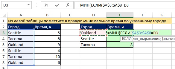
Rice. 4.4. Create an array operator in an argument log_expression IF functions
So you've created an array operator with a comparison operator. At any time during array processing, the array operator is a comparison operator, so its result will be an array of TRUE and FALSE values. To verify this, select the array (to do this, click on the argument in the tooltip log_expression) and press F9 (Fig. 4.5). Usually you use one argument log_expression, returning either TRUE or FALSE; here, the resulting array will return multiple TRUE and FALSE values, so the MIN function will select the minimum number only for those cities that match the TRUE value.

Rice. 4.5. To see an array of TRUE and FALSE values, click the argument in the tooltip log_expression and press F9